How to Regularize your LoRA Training Better
Six ways to add dropout-style noise to LoRA fine-tuning, compared across three datasets, two base models and five seeds. One of them, Drop-LoRA-Path, beats standard LoRA dropout and weight decay in every comparison.
Introduction
A year ago, while running supervised classification fine-tuning for ExPLoRA (ICML 2025)
We note that the original LoRA configuration outperforms other PEFT techniques when paired with the drop-path regularization technique
But this has remained a small itch that I’ve wanted to scratch. And so a year later, now armed with my own DGX Spark, I thought I’d test this appendix note’s generalizability to language models. It strikes me as weird - drop-path is essentially zeroing out the entire result of one layer’s contribution to the model’s residual path. Isn’t it too aggressive for low-rank fine-tuning? Why does it work better than vanilla dropout and why isn’t this a standard regularization tool for LoRA?
So this exploration is what came of pulling that thread. In this blog, we’ll aim to answer a few questions -
- Does the pattern I saw in vision transfer to language modeling?
- Does this “drop-path” regularization beat weight decay and LoRA dropout?
- Why does it work? Can we find basic mechanistic explanations?
To answer these questions, we’ll pretrain 286M parameter language models, define a ‘regularization ladder’ of six variants that change where and how the noise is applied, and sweep them across three downstream datasets. The variant we’ll call “drop-LoRA-path” consistently wins across all configurations. If you LoRA fine-tune, this is worth a try!
TL;DR
- We construct a regularization ladder, exploring the effects of the placement and granularity of dropout/drop-path style regularization on LoRA training.
- Drop-LoRA-Path (DLP), drop-path on the LoRA branch alone, beats standard LoRA dropout and weight decay in all 30 comparisons (3 datasets × 5 seeds × 2 base models). The margin over LoRA dropout is consistent (1.4% in val. loss, ~1% in perplexity).
- We find that DLP is better at preventing the fine-tuned model from drifting from the base as it learns and at mitigating co-adaptation than dropout and other LoRA regularization methods.
If your LoRA fine-tune overfits, replace lora_dropout with DLP at a drop rate of 0.3, the same in every layer. It costs nothing at inference!
Code: github.com/samar-khanna/lora-regularization
Background
Low-rank adaptation (LoRA)
Fine-tuning every weight of a large model is expensive, so LoRA
where \(A \in \mathbb{R}^{r \times k}\) and \(B \in \mathbb{R}^{d \times r}\) are the only trainable parameters, structured as low-rank matrices with rank \(r \ll \min(d, k)\), and \(\alpha\) is a fixed scale. \(A\) is initialized randomly and \(B\) to zero, so the adapter starts as a no-op and fine-tuning begins exactly at the pretrained model.
Why regularize LoRA?
A low-rank update is itself a form of regularization, as it limits the degrees of freedom with which the model can move. However, it does not prevent overfitting. Fine-tuning data for a specific task or domain is often small, consisting of a few thousand to tens of thousands of high-quality examples
Dropout and drop-path
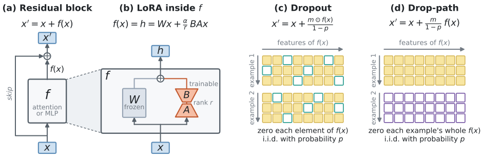
A transformer is a stack of residual blocks. Each block adds the output of a branch \(f\), an attention or MLP sublayer, to the residual stream (Figure 1a):
\[x' = x + f(x), \qquad x,\, f(x) \in \mathbb{R}^{L \times d},\]where each example \(x\) consists of \(L\) tokens’ hidden states, each of dimension \(d\). The linear maps that LoRA adapts live inside these branches and act on each token separately (Figure 1b). Dropout and drop-path both regularize this update by zeroing parts of \(f(x)\) at random during training. They differ in which parts they zero.
Dropout
where \(\odot\) is element-wise multiplication. A new mask is drawn for every example.
Drop-path, also called stochastic depth
where the single mask value \(m\) is drawn per example and shared by all of its tokens. With probability \(p\) the block is skipped for that example. Drop-path is standard when training and fine-tuning ViTs
Each training step therefore trains a random sub-network: dropout removes individual units, and drop-path removes whole blocks. The noise prevents parts of the network from relying too much on each other, forcing these parts to learn updates that are useful on their own. Under dropout, a unit cannot rely on any specific other unit being present. Under drop-path, a block cannot rely on the blocks before it having run. This can prevent co-adaptation in deep networks, as it helps each block individually contribute. At inference the full network runs, and it behaves roughly like an average over all of these sub-networks
Figure 2 shows these sub-networks on a toy problem.
The LoRA regularization ladder
Rather than only compare standard LoRA dropout and drop-path, for this post I wanted to examine the regularization choices on the residual path more closely. Standard LoRA dropout and drop-path differ in two ways: where the noise goes, and whether it is applied per element or per example. Dropout acts on the adapter’s input, one element at a time, along the feature dimension of a token’s hidden state. Drop-path acts on the whole branch, one example at a time, as a binary choice determining whether the branch’s output is kept or dropped, usually for all of that example’s tokens. Varying both gives a ladder of six regularizers (Figure 3). Each rung changes one thing from the rung below: L1–L3 move element-wise dropout from the adapter’s input to its output, L3–L5 keep the noise on the adapter’s output and coarsen the mask from one value per element to one per token to one per sequence, and L6 extends drop-path from the adapter to the whole branch.
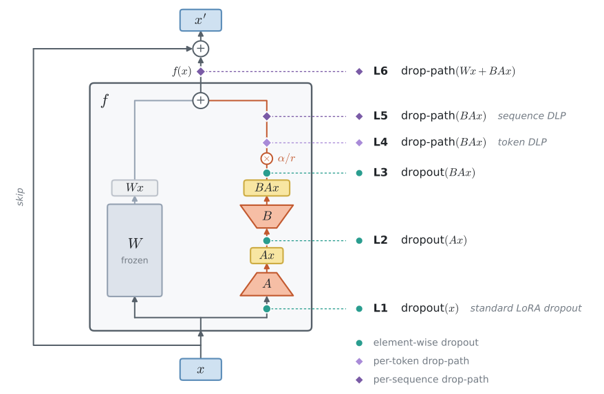
To make this explicit, write \(m \sim \mathrm{Bernoulli}(1-p)\) for a random mask (i.e. entries are 1 with probability \(1-p\) and 0 otherwise), broadcast over any dimension its shape lacks. Leaving out the \(\alpha/r\) scale and the division by \(1-p\), each rung on the ladder computes:
| Rung | Name | Computation during training | Mask \(m\) | Noise |
|---|---|---|---|---|
| L0 | none | \(f(x) = Wx + BAx\) | — | none |
| L1 | dropout\((x)\) | \(f(x) = Wx + BA\,(m \odot x)\) | \(\{0,1\}^{L \times k}\) | per element |
| L2 | dropout\((Ax)\) | \(f(x) = Wx + B\,(m \odot Ax)\) | \(\{0,1\}^{L \times r}\) | per element |
| L3 | dropout\((BAx)\) | \(f(x) = Wx + m \odot BAx\) | \(\{0,1\}^{L \times d}\) | per element |
| L4 | token DLP | \(f(x) = Wx + m \odot BAx\) | \(\{0,1\}^{L}\) | per token |
| L5 | sequence DLP | \(f(x) = Wx + m \odot BAx\) | \(\{0,1\}\) | per sequence |
| L6 | drop-path\((Wx+BAx)\) | \(x' = x + m \odot f(x)\) | \(\{0,1\}\) | per sequence |
- L1 is standard LoRA dropout:
lora_dropoutin Hugging Face PEFT and in the original LoRA code. The frozen path \(Wx\) still sees the clean input. - L2 drops coordinates of the rank-\(r\) bottleneck. It matches DropLoRA
and the network_dropoutoption of the Stable Diffusion LoRA trainer sd-scripts. - L3 applies dropout to the adapter’s output. It is the element-wise counterpart of L4 and L5.
- L4 is token DLP. Drop-LoRA-Path (DLP) applies drop-path to the adapter’s residual path alone, and token DLP draws one mask value per token: within a sequence, some tokens get a layer’s adapter update and others don’t.
- L5 is sequence DLP, which draws one mask value per sequence. For each sequence and each adapted layer, with probability \(p\) the layer computes only \(Wx\) for every token, exactly as the frozen model would. Elsewhere in this post, DLP on its own means sequence DLP.
- L6 is ordinary drop-path during fine-tuning, as in ViT recipes. The whole branch \(f\) is dropped, frozen weights and adapters together. Its rate rises linearly with depth, from 0 in the first block to \(p\) in the last.
We leave out two whole-branch variants: a per-token version of L6, and element-wise dropout on \(f(x)\) as in Figure 1(c), the residual dropout of the original Transformer. Unlike L1–L5, both add noise to the frozen path, so their effect depends on how the base model was pretrained. As we'll see, L6 works poorly unless the base model was pretrained with drop-path, so a fair test of either would need its own pretrained base model.
All six act only during training. At inference the adapter runs in full and can be merged into \(W\) as usual.
Example DLP implementation
DLP (implemented below as L5) takes a few lines, where L4 and L5 differ only in the mask’s shape, (batch, seq, 1) versus (batch, 1, 1):
class LoRALinear(nn.Module):
    def __init__(self, base: nn.Linear, rank=32, alpha=32, p=0.3):
        super().__init__()
        self.base = base.requires_grad_(False)                # frozen W
        bound = 1 / base.in_features ** 0.5
        self.A = nn.Parameter(torch.empty(rank, base.in_features).uniform_(-bound, bound))
        self.B = nn.Parameter(torch.zeros(base.out_features, rank))
        self.scale, self.p = alpha / rank, p

    def forward(self, x):                                     # x: (batch, seq, in_features)
        delta = (x @ self.A.T) @ self.B.T                     # BAx
        if self.training and self.p > 0:                      # Drop-LoRA-Path:
            keep = torch.rand(x.shape[0], 1, 1, device=x.device) >= self.p   # one coin per sequence
            delta = delta * keep / (1 - self.p)
        return self.base(x) + self.scale * delta
In summary, the regularization ladder allows us to vary the granularity and placement of activation noise along the residual path. Compared with standard LoRA dropout, DLP changes two things: which tensor is masked (BAx instead of x) and the shape of the mask (one value per example instead of one per element).
Setup
Base models. I pretrained two 12-layer Llama-style models with nanochat. Each has 286M parameters, of which 110M are non-embedding parameters. Both were trained on 2.2B tokens of FineWeb-Edu
LoRA. Rank 32 and \(\alpha = 32\) on all six linear maps of every block (query, key, value, attention output and both MLP projections). AdamW with learning rate \(3 \times 10^{-3}\), effective batch size 16, and 4,500 steps on a cosine schedule. The loss covers response tokens only. These settings came from a 96-run sweep without regularization over adapter placement, rank, learning rate and batch size, guided by Thinking Machines’ LoRA Without Regret (Appendix B).
Datasets. Three supervised fine-tuning tasks, each small enough that 4,500 steps covers it several times:
| Dataset | Task | Train / val examples | Epochs in 4,500 steps |
|---|---|---|---|
| OpenCodeReasoning, HackerEarth subset | competitive programming with reasoning and solutions, split 90/10 by problem | ~11.2K / ~1.2K | ~6.4 |
| GSM8K | grade-school math word problems with worked solutions | 7,473 / 1,319 | ~9.6 |
| Glaive function calling v2 | first-turn function-calling conversations with responses of at least 100 tokens, 10K subsample | 9,000 / 1,000 | 8.0 |
The datasets cover domains that may not be strongly represented in the pretraining data. For example, Glaive’s JSON function-call format barely appears in FineWeb-Edu, so the model has to learn something new rather than recall it.
Protocol. Each ladder rung was swept over \(p \in \{0.05, 0.1, 0.2, 0.3\}\), with the same rate in every transformer layer except for L6, which uses the linear depth schedule (for parity with ViTs). AdamW’s decoupled weight decay on \(A\) and \(B\) (no dropout) was swept over \(\{0.01, 0.05, 0.1, 0.2, 0.3, 0.4\}\). I ran every configuration with 5 seeds on 3 datasets and both base models, totaling 930 fine-tuning runs.
The metric used is the best average validation loss (cross-entropy on response tokens, in nats)
Results
LoRA overfits without regularization
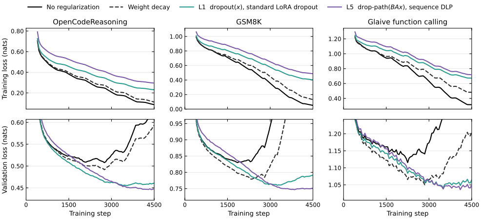
Figure 4 motivates the problem we are trying to solve. Without regularization, LoRA overfits: validation loss traces a signature U-curve around four epochs in (1,850 to 2,750 steps, depending on the dataset). Even as training loss keeps falling, validation loss climbs steeply with more passes over the dataset. The best weight decay value partly delays overfitting, but does not fully mitigate it on any of the three datasets. On the other hand, both dropout-style regularizers keep validation loss falling longer. Standard LoRA dropout reaches its best around step 3,400, and DLP around step 4,000.
Drop-LoRA-Path (DLP) is the best rung on the regularization ladder
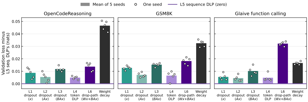
Given the significance of regularization in preventing overfitting, Figure 5 compares the rungs of the LoRA regularization ladder, across 3 datasets and 5 seeds. Sequence DLP (L5) has the lowest validation loss, on every dataset (Figure 5). It beats standard LoRA dropout in all 15 pairs on each base, by 0.009 nats on average (1.4%, about 1% in perplexity). Token DLP (L4) is next, which reinforces the regularizing benefits of drop-path on the LoRA residual path. Of the other rungs, dropout\((Ax)\) (L2) comes closest. Weight decay trails DLP by 0.03 nats (5.5%) on average, even with its best value picked separately for every seed.
Paired comparisons with DLP on the standard base
| Compared with DLP | DLP better in | Mean gap (nats) |
|---|---|---|
| No regularization | 15/15 | 0.075 |
| L1 dropout\((x)\), standard | 15/15 | 0.009 |
| L2 dropout\((Ax)\) | 15/15 | 0.006 |
| L3 dropout\((BAx)\) | 15/15 | 0.012 |
| L4 token DLP | 15/15 | 0.005 |
| L6 drop-path\((Wx+BAx)\) | 15/15 | 0.021 |
| Weight decay | 15/15 | 0.032 |
Pairs are dataset × seed. Every comparison has \(p = 3 \times 10^{-5}\) (one-sided Wilcoxon signed-rank), the smallest possible value with 15 pairs, so correcting for multiple comparisons would not change any conclusion. Confidence intervals, absolute losses and the drop-path base are in Appendix C.
For scale, DLP lowers validation loss relative to no regularization by 0.060, 0.083 and 0.082 nats on OpenCodeReasoning, GSM8K and Glaive (7–12%, 6–8% in perplexity).
DLP’s lead grows with the drop rate
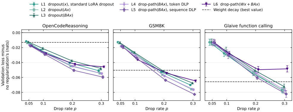
At \(p \le 0.1\) the rungs are close, and from \(p = 0.2\) on DLP is ahead on every dataset (Figure 6). On the standard base, DLP beats standard dropout in 12, 13, 15 and 15 of the 15 pairs at the four rates. Averaged over the four rates, it beats standard dropout across all 15 pairs, so the result doesn’t depend on a single well-chosen rate.
Weight decay at its best value is worth about as much as standard dropout at \(p = 0.2\) on GSM8K, between \(p = 0.2\) and \(0.3\) on Glaive, and only \(p = 0.05\) on OpenCodeReasoning.
For an additional ablation that tests the impact of changing the drop-path rate per layer, you can review Appendix D. The result confirms the default choice of keeping the same rate in every layer, which works best.
Full drop-path (L6) needs a base model pretrained with it
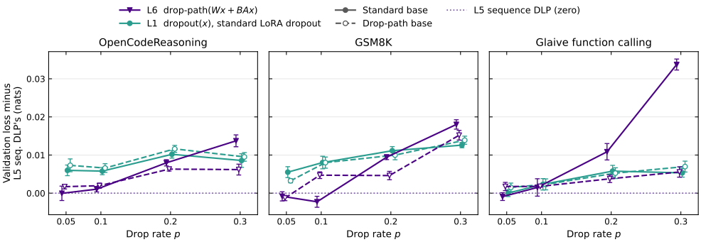
So far, I haven’t directly reproduced my original finding in ExPLoRA
To test this hypothesis, I trained the drop-path base. If it is right, L6 should catch up on this base. It partly does. At its best rate, its gap to DLP shrinks from 0.021 to 0.009 nats (2.9% to 1.3%)
However, the drop-path base does not seem to be a better starting point overall. Its best result per dataset and seed is 0.006 nats (0.7%) worse than the standard base’s on average. I use it only as a probe. For LoRA regularization specifically, L6 on either base is fine at low rates, where it roughly ties DLP at \(p \le 0.1\). In summary, DLP remains the preferred regularization method, where its wins are agnostic to the base’s pretraining.
Why does Drop-LoRA-Path work?
The intuition we can build on is this: when DLP drops an adapter, that layer computes exactly what the base model would for the whole example. So every training step runs a network that is partly the base model. The noise is also correlated across every token and feature of an adapter’s output. This has three testable effects: the fine-tuned model stays close to the base model, each adapter has to learn an update that works without the others, and training penalizes interactions between the entries of each adapter’s output. Unless noted, the measurements in this section use the adapters at the end of training on all three datasets, on the standard base, with every dropout-style rung at \(p = 0.3\).
DLP forgets the least
Of all the methods, DLP changes the base model’s behavior on general text the least (Figure 8).
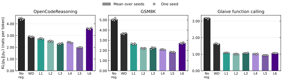
Fine-tuning costs a model some of its general ability
DLP’s forgetting levels off
Here we plot \(\mathrm{KL}(p_\theta \,\Vert\, p_{\theta'})\) as before against next-token prediction accuracy on each dataset’s validation split, over the course of training. Standard dropout keeps forgetting as it learns (higher KL), while DLP’s forgetting levels off (Figure 9).
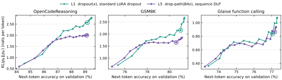
For example, on GSM8K below about 78% accuracy the two curves are close. After that, standard dropout’s KL keeps rising with each point of accuracy, while DLP’s stays near 1.7. OpenCodeReasoning shows the same pattern, with DLP’s KL leveling off near 2.0. On Glaive the two curves stay close, and both rise in the last stretch of training.
DLP prevents the adapters from co-adapting
To measure co-adaptation, for each method we drop all but one transformer block’s 6 trained adapters and measure the resulting model’s validation loss minus the base model’s per dataset. Without regularization, the adapters in the last block are the weakest on their own across datasets. Under DLP, every block’s adapters work on their own (Figure 10).
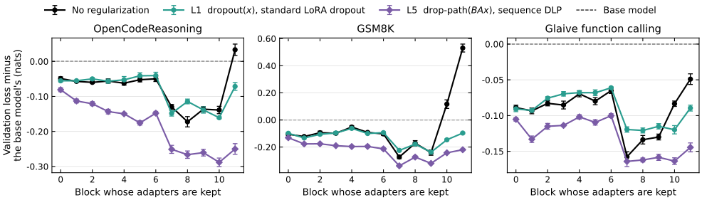
On GSM8K and Glaive the last two blocks are harmful in the full model too: removing either one’s adapters lowers the unregularized model’s validation loss by 0.10–0.23 nats (7–15%). Both dropout rungs remove this, and DLP’s blocks are the most useful alone: on average a single DLP block lowers validation loss by 0.18 nats (8.7%), against 0.10 (4.8%) for standard dropout.
Appendix E shows the results of swapping blocks of adapters between two separately trained runs of the same method, differing in seed. DLP is more robust to these swaps than standard dropout or no regularization.
DLP penalizes interactions within each adapter’s output
Staying close to the base model doesn’t explain the whole ladder, though. L3 drifts less from the base than standard dropout on OpenCodeReasoning and GSM8K (Figure 8), yet its validation loss is worse. L3, L4 and L5 put noise on the same tensor, \(BAx\), and differ only in the shape of the mask, yet DLP beats L3 in all 15 pairs (Figure 5). To understand why, we can expand the loss to second order to show what the mask shape changes: DLP’s mask penalizes interactions between entries of the adapter update \(BAx\), and L3’s mask cannot.
Recall, without noise, a block computes
\[x' = x + Wx + BAx\]where we assume \(f\) is a single linear map as in Figure 1. L3, L4 and L5 multiply only the adapter’s term by the mask, so during training the block computes
\[\tilde{x}' = x + Wx + \frac{m}{1-p} \odot BAx,\]where, as in the ladder, \(m \in \{0, 1\}^{L\times d}\) for L3, \(m \in \{0, 1\}^L\) for L4, and \(m \in \{0,1 \}\) for L5. Taking the difference of the noisy and noise-free outputs, the noise shifts the block’s output by
\[\delta = \tilde{x}' - x' = \epsilon \odot BAx, \qquad \epsilon = \frac{m}{1-p} - 1 .\]Each entry of \(\epsilon\) is \(-1\) with probability \(p\), when the update is dropped, and \(\frac{p}{1-p}\) otherwise, so it has mean \(\mathbb{E}_m[\epsilon_i] = 0\) and variance \(\text{Var}_m[\epsilon_i] = \sigma^2 = \frac{p}{1-p}\).
Let \(\ell\) be one example’s loss as a function of the block’s output \(x'\), with gradient \(\nabla \ell\) and Hessian \(H\) at \(x'\), treating \(x', BAx \in \mathbb{R}^{Ld}\) (flattened vectors of \(Ld\) entries). Expanding the loss averaged over masks to second order gives
\[\begin{aligned} \mathbb{E}_m\big[\ell(\tilde{x}')\big] & = \mathbb{E}_m\big[\ell(x' + \delta)\big] \\ &\approx \ell(x') + \nabla\ell^\top\, \mathbb{E}_m[\delta] + \tfrac{1}{2}\, \mathbb{E}_m\big[\delta^\top H \delta\big] \\ &= \ell(x') + \underbrace{\tfrac{1}{2} \textstyle\sum_{i,j} H_{ij}\, (BAx)_i\, (BAx)_j\, \mathbb{E}_m[\epsilon_i\, \epsilon_j]}_{\Omega(x)}, \end{aligned}\]since \(\mathbb{E}_m[\delta] = 0\). Training with the noise therefore minimizes the clean loss plus the last term \(\Omega(x)\), a penalty
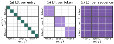
With \(BAx\) flattened token by token, token \(t\) holds entries \((t-1)d+1\) to \(td\), and the penalty for each rung is
\[\begin{aligned} \Omega_{\text{L3}}(x) &= \frac{\sigma^2}{2} \sum_{i=1}^{Ld} H_{ii}\, (BAx)_i^2, \\ \Omega_{\text{L4}}(x) &= \frac{\sigma^2}{2} \sum_{t=1}^{L}\, \sum_{i,j=(t-1)d+1}^{td} H_{ij}\, (BAx)_i\, (BAx)_j, \\ \Omega_{\text{L5}}(x) &= \frac{\sigma^2}{2} \sum_{i,j=1}^{Ld} H_{ij}\, (BAx)_i\, (BAx)_j. \end{aligned} \tag{1}\]\(\Omega_{\text{L3}}\) counts each entry on its own, \(\Omega_{\text{L4}}\) adds every pair of entries in the same token, and \(\Omega_{\text{L5}}\) adds every pair of entries in the sequence.
For two entries \(i \neq j\), the pair term is their interaction. To second order,
\[H_{ij}\,(BAx)_i\,(BAx)_j \approx \Delta\ell_{i,j} - \Delta\ell_i - \Delta\ell_j ,\]where \(\Delta\ell = \ell(x'+\delta) - \ell(x')\), \(\Delta\ell_i\) is the rise in loss from dropping entry \(i\) of \(BAx\) alone, and \(\Delta\ell_{i,j}\) the rise from dropping entries \(i\) and \(j\) together.
Each penalty can be measured on a trained model. We can switch on a rung’s noise at \(p=0.3\) in every adapter, as during training, and record how much the training loss rises averaged over 64 training examples and fresh masks drawn for each. By the expansion above, this is \(\Omega\) averaged over those example sequences. The masks of the 72 adapters across the transformer are independent, so this rise is the sum of their penalties. We can thus compute \(\Omega_{\text{L3}}\), \(\Omega_{\text{L4}}\) and \(\Omega_{\text{L5}}\), and \(\Omega_{\text{L5}} - \Omega_{\text{L3}}\) leaves only the non-diagonal pair terms. Figure 12 compares all four with each rung’s validation loss.
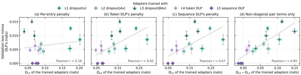
There is a clear correlation between the pair terms a rung leaves in its adapters and its validation loss.
Appendix F tracks the pair terms over training: DLP removes them as it trains, while standard dropout’s stay near their early level. Appendix G demonstrates that Gaussian noise with the same shape, which doesn’t drop adapter outputs, performs the same as DLP.
Discussion
When should you use drop-LoRA-path?
My biggest takeaway is that LoRA fine-tuning can be heavily under-regularized. As we’ve seen, validation loss can improve a lot with heavier regularization (of any type) when training for multiple epochs. Simply raising the regularization rate from 0.05 to 0.3 increases the gain in validation loss over no regularization from 1.7% to 8.5% for standard dropout, and from 2.3% to 9.7% for DLP. My second takeaway is that DLP was the best regularizer in this post, and it beat standard dropout on every dataset, base model and seed, with no cost to inference. So if your LoRA fine-tuning on a small dataset overfits within your training budget, replace lora_dropout with DLP at \(p=0.3\), with the same rate in every layer. However, if your fine-tuning budget is smaller and covers one or two epochs, you can likely use weight decay, standard dropout, or DLP at a lower rate.
Related work
Stochastic depth on adapters has precedent in vision. Adapters Strike Backmodule_dropout option that skips whole LoRA modules. sd-scripts draws one coin per batch rather than per example and does not rescale.
For LoRA on language models, prior work on dropout varies where in the transformer to drop (HiddenKey
Don’t Drop Dropout
Limitations
- Small model experiments. Everything uses a 286M-parameter, 12-layer model pretrained from scratch, not an off-the-shelf LLM.
- Validation loss only. A model this small can’t meaningfully solve GSM8K or competitive programming problems, so I didn’t measure task accuracy. As in LoRA Without Regret
, I compare methods by log loss rather than sampling-based evals, since it gives clean comparisons across training settings. - Hyperparameters. To balance spending more compute with achieving lower validation loss, drop rates stop at 0.3 in these experiments. Results may differ at higher rates. The best LoRA configuration (rank, batch size etc.) was also selected via a sweep before the regularization analysis, and different configurations may also influence results.
Open questions
- Can we reproduce these results on open-source LLMs in the 0.5–1B range or larger?
- Can we construct a longer regularization ladder including additional techniques for a broader analysis?
- How do other regularization techniques like KL regularization combine with dropout/drop-path during training?
Appendix
A. Pretraining
Pretraining curves for the two base models
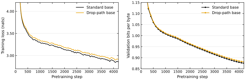
Both models ran 4,200 steps of 524,288 tokens (2.2B tokens). The drop-path base’s training loss is higher because drop-path is active during training. Its validation loss, measured without drop-path, ends close to the standard base’s: 0.881 versus 0.875 bits per byte. On nanochat’s CORE evaluation the drop-path base scores 0.153 and the standard base 0.147.
B. LoRA hyperparameters
LoRA hyperparameter sweep
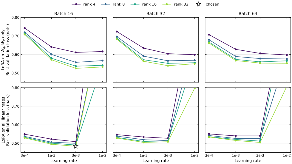
The sweep covered adapter placement (query and value maps only, or all six linear maps) × rank {4, 8, 16, 32} × learning rate {3e-4, 1e-3, 3e-3, 1e-2} × effective batch size {16, 32, 64}, 96 runs in total. LoRA on all linear maps beats query and value only at every rank, by a wide margin, as LoRA Without Regret also found. Higher rank helps at every stable learning rate, and batch 16 beats larger batches in every case but one: query and value only at rank 4, where batch 64 is slightly better. The best run, rank 32 on all linear maps at learning rate 3e-3 and batch 16, is the configuration used throughout.
C. Per-dataset results
Absolute validation loss and confidence intervals
Standard base
| OpenCodeReasoning | GSM8K | Glaive | |
|---|---|---|---|
| L0 none | 0.505 ± 0.028 | 0.828 ± 0.003 | 1.114 ± 0.008 |
| L1 dropout\((x)\), standard | 0.454 ± 0.027 | 0.758 ± 0.003 | 1.037 ± 0.004 |
| L2 dropout\((Ax)\) | 0.450 ± 0.026 | 0.753 ± 0.002 | 1.036 ± 0.003 |
| L3 dropout\((BAx)\) | 0.457 ± 0.026 | 0.761 ± 0.002 | 1.041 ± 0.005 |
| L4 drop-path\((BAx)\), token DLP | 0.450 ± 0.025 | 0.752 ± 0.004 | 1.036 ± 0.003 |
| L5 drop-path\((BAx)\), sequence DLP | 0.445 ± 0.025 | 0.746 ± 0.002 | 1.031 ± 0.004 |
| L6 drop-path\((Wx+BAx)\) | 0.459 ± 0.027 | 0.764 ± 0.002 | 1.063 ± 0.003 |
| Weight decay | 0.492 ± 0.026 | 0.778 ± 0.004 | 1.048 ± 0.003 |
Drop-path base
| OpenCodeReasoning | GSM8K | Glaive | |
|---|---|---|---|
| L0 none | 0.507 ± 0.029 | 0.830 ± 0.003 | 1.124 ± 0.008 |
| L1 dropout\((x)\), standard | 0.456 ± 0.026 | 0.765 ± 0.003 | 1.048 ± 0.003 |
| L2 dropout\((Ax)\) | 0.455 ± 0.026 | 0.759 ± 0.001 | 1.044 ± 0.002 |
| L3 dropout\((BAx)\) | 0.461 ± 0.027 | 0.769 ± 0.001 | 1.051 ± 0.003 |
| L4 drop-path\((BAx)\), token DLP | 0.452 ± 0.025 | 0.758 ± 0.002 | 1.047 ± 0.003 |
| L5 drop-path\((BAx)\), sequence DLP | 0.447 ± 0.027 | 0.751 ± 0.001 | 1.041 ± 0.004 |
| L6 drop-path\((Wx+BAx)\) | 0.453 ± 0.026 | 0.767 ± 0.003 | 1.046 ± 0.003 |
| Weight decay | 0.495 ± 0.027 | 0.782 ± 0.002 | 1.056 ± 0.006 |
Mean ± standard deviation over 5 seeds, each method at its best grid value. The standard deviations are large on OpenCodeReasoning because each seed holds out a different validation split. The paired gaps below remove that variation.
| Compared with DLP | Standard base: mean gap [95% CI] | Drop-path base: mean gap [95% CI] |
|---|---|---|
| No regularization | 0.0748 [0.0678, 0.0818] | 0.0741 [0.0675, 0.0807] |
| L1 dropout\((x)\), standard | 0.0088 [0.0066, 0.0111] | 0.0101 [0.0080, 0.0123] |
| L2 dropout\((Ax)\) | 0.0055 [0.0040, 0.0071] | 0.0063 [0.0048, 0.0078] |
| L3 dropout\((BAx)\) | 0.0123 [0.0105, 0.0140] | 0.0139 [0.0115, 0.0162] |
| L4 drop-path\((BAx)\), token DLP | 0.0053 [0.0037, 0.0068] | 0.0063 [0.0050, 0.0075] |
| L6 drop-path\((Wx+BAx)\) | 0.0212 [0.0165, 0.0259] | 0.0090 [0.0060, 0.0119] |
| Weight decay | 0.0317 [0.0246, 0.0389] | 0.0314 [0.0235, 0.0393] |
Gaps are the method’s validation loss minus DLP’s in nats, averaged over 15 dataset-seed pairs, with t-based 95% confidence intervals.
D. Drop rate across layers
Uniform, ascending and descending DLP rate schedules
All DLP results in the main text use the same rate in every layer, while ordinary drop-path ramps the rate up with depth. To test whether the schedule matters for DLP, I reran it on the standard base (3 seeds, \(p \in \{0.1, 0.2, 0.3\}\)) with the rate rising linearly from 0 in the first layer to \(p\) in the last (ascending), or falling from \(p\) to 0 (descending). Each schedule gets its best peak rate.
| Schedule | Validation loss minus uniform’s (nats) | Uniform better in |
|---|---|---|
| Ascending, 0 → \(p\) | +0.017 | 9/9 pairs |
| Descending, \(p\) → 0 | +0.061 | 9/9 pairs |
Part of uniform’s advantage is that it applies twice the average noise at the same peak rate. Ascending and descending apply the same average noise, yet ascending beats descending in all 9 pairs, by 0.044 nats (6.6%). Heavy noise in the early layers hurts. Uniform is a good default.
E. Swapping adapters between training runs
Hybrids built from two training runs of the same method
This test of co-adaptation swaps adapters between training runs. We train the same method twice with different seeds, then build a hybrid from the first run’s adapters in blocks 0–5 and the second run’s in blocks 6–11. If each block’s update is individually useful, the hybrid works about as well as the two originals; if the blocks are co-dependent, the hybrid would have worse validation loss (Figure E1).
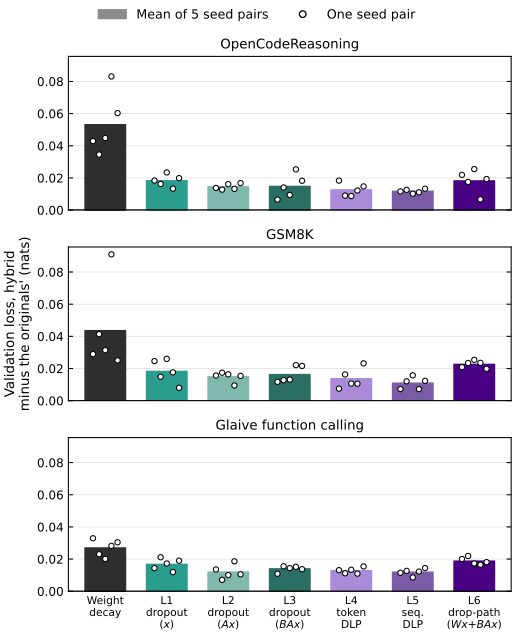
On all three datasets, the hybrid’s validation loss is 0.06–0.09 nats (4–11%) worse than the originals’ without regularization, 0.017–0.018 (2–4%) worse with standard dropout, and only 0.011–0.012 (1–3%) worse with DLP.
F. Pair terms over training
Pair terms at each checkpoint for standard dropout and DLP
The pair terms in Figure 12 were measured at the end of training. Figure F1 tracks them through training, on the checkpointed reruns of standard dropout and DLP used for Figure 9.
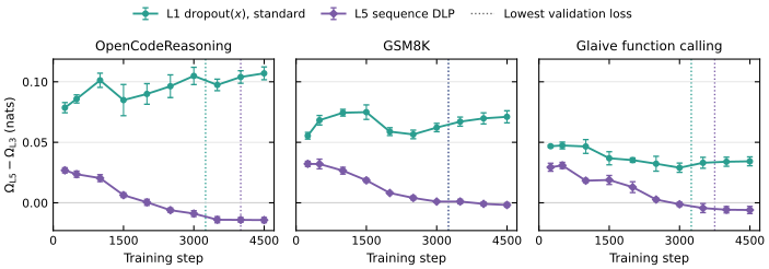
Standard dropout’s pair terms are there from the first checkpoint and stay near that level through training, including after its validation loss turns up. DLP’s start lower and fall to about zero by step 2,500. The gap in Figure 12 comes from DLP removing the pair terms as it trains, not from standard dropout accumulating them as it overfits.
G. Gaussian noise with DLP’s shape
DLP’s noise shape without dropping the adapter
DLP’s mask does two things: it removes an adapter’s whole output, so the layer computes what the base model would, and it shares one noise value across every token and feature of that output. To separate the two, I replaced DLP’s keep/drop factor \(m/(1-p)\) with a Gaussian factor \(g \sim \mathcal{N}\big(1, \tfrac{p}{1-p}\big)\), drawn the same way: once per sequence for each adapter. The noise \(g - 1\) has the same mean and variance as DLP’s \(\epsilon\), so the expansion in the main text gives the same penalty \(\Omega_{\text{L5}}\), but the adapter is never removed (about 6% of draws are negative and flip the adapter’s update for that sequence). This is Gaussian dropout
| Compared with Gaussian DLP | Mean gap (nats) | Gaussian DLP better in |
|---|---|---|
| L1 dropout\((x)\), standard | 0.0098 | 15/15 |
| L2 dropout\((Ax)\) | 0.0065 | 14/15 |
| L3 dropout\((BAx)\) | 0.0133 | 15/15 |
| L4 drop-path\((BAx)\), token DLP | 0.0062 | 15/15 |
| L5 drop-path\((BAx)\), sequence DLP | 0.0010 | 9/15 |
Gaps are each method’s validation loss minus Gaussian DLP’s, averaged over 15 dataset-seed pairs, with every method at \(p = 0.3\).
Gaussian DLP matches DLP (two-sided Wilcoxon \(p = 0.19\)) and beats L3 in all 15 pairs, although L3 puts noise of the same variance on each entry of \(BAx\). So DLP’s advantage over L3 comes more from sharing noise across the adapter’s output than from removing the adapter. This is what the pair terms in the penalty capture.
Citation
Please cite this work as:
Khanna, Samar. “How to Regularize your LoRA Training Better.” samar-khanna.github.io, November 2026. https://samar-khanna.github.io/blog/2026/lora-regularization/
Or use the BibTeX citation:
@misc{khanna2026lorareg,
  author = {Khanna, Samar},
  title  = {How to Regularize your {LoRA} Training Better},
  year   = {2026},
  month  = nov,
  url    = {https://samar-khanna.github.io/blog/2026/lora-regularization/},
  note   = {Blog post}
}